You Need 400 Years of Data to Estimate an Expected Return

A quant can measure the volatility of a stock to four decimal places from one year of intraday data. Measuring its expected return to within one percentage point takes four hundred years.

Both numbers come from the same model, the same price series and the same estimator. The asymmetry is not a data problem, and no amount of computing power or sampling frequency closes it. It is structural, and it explains more about how derivatives desks work than almost anything else in the toolkit.

The arithmetic

Take geometric Brownian motion, the simplest possible setting:

$\frac{dS_t}{S_t} = \mu dt + \sigma dW_t$

Observe the price over $T$ years. The natural estimator of the drift is the total log return, annualised and corrected for the Itô term. Its standard error is

$\mathrm{se}(\hat{\mu}) = \frac{\sigma}{\sqrt{T}}$

Look carefully at what is missing from that expression. There is no $n$ . The number of observations does not appear. Only $T$ , the calendar length of the window.

With a typical equity volatility of 20%:

Sample length	Standard error of $\hat{\mu}$
1 year	20.00%
5 years	8.94%
10 years	6.32%
36 years	3.33%
100 years	2.00%
400 years	1.00%

Inverting it gives the headline. A standard error of five percentage points needs 16 years. Two percentage points needs a century. One percentage point needs 400 years. Half a point needs 1,600.

For context: the entire post-war history of the S&P 500 is shorter than the window required to say whether the equity risk premium is 5% or 7%.

Sampling faster does not help. At all.

The obvious objection is that nobody uses annual data any more. We have tick data. Surely a year sampled every minute carries more information than a year sampled monthly.

It does — about volatility. It carries exactly the same information about the drift. Simulate a year of GBM with $\mu = 8\%$ and $\sigma = 20\%$ , three thousand paths, at four sampling frequencies, and measure how much the two estimates bounce around:

Observations per year	sd of $\hat{\mu}$	sd of $\hat{\sigma}$
12 (monthly)	19.96%	4.111%
252 (daily)	19.82%	0.885%
2,016 (hourly)	20.03%	0.316%
120,960 (per minute)	19.98%	0.041%

Going from monthly to minute data is a ten-thousand-fold increase in observations. The volatility estimate improves by a factor of a hundred, exactly the $1/\sqrt{2n}$ the theory predicts. The drift estimate does not improve at all. It sits at 20% in every row, because $\sigma/\sqrt{T}$ with $T = 1$ is 20% and nothing else enters.

This is worth stating in the strongest form. Every tick of intraday data you have ever collected contains precisely zero information about expected return beyond what the first and last prices of the window already told you. The drift estimator depends on the sample only through $\log S_T - \log S_0$ . Everything in between cancels.

Why the two parameters behave so differently

The mechanism is the quadratic variation of the path.

Volatility shows up in the sum of squared increments. Over a window of length $T$ with $n$ steps, that sum converges to $\sigma^2 T$ as $n$ grows, and it converges pathwise — for the one path you actually observed, not on average across paths you did not. In the continuous limit, $\sigma$ is not estimated at all. It is read off the path. The quadratic variation of $\log S$ over $[0,T]$ equals $\sigma^2 T$ with probability one.

The drift shows up in the sum of the increments themselves, which telescopes to the endpoints. Refining the grid adds terms that cancel. There is nothing to accumulate.

The sharpest way to say this comes from Girsanov’s theorem. Changing the drift of a diffusion produces a new measure that is equivalent to the original one over any finite horizon: the two assign positive probability to exactly the same sets of paths. A world where the stock drifts at 2% and a world where it drifts at 12% are mutually absolutely continuous. No finite observation, at any frequency, can rule either out.

The volatility is different precisely because an equivalent change of measure leaves the quadratic variation untouched. Girsanov moves the drift and never touches $\sigma$ . That is the same fact seen from the other side: $\sigma$ is a property of the path, $\mu$ is a property of the measure, and you only ever observe one path.

So this is not a small-sample problem waiting for a better estimator. The drift is not identified.

What it costs in practice

Three consequences that cause real damage.

Fund selection is mostly noise. Take two managers whose true expected returns genuinely differ by two percentage points, 8% against 6%, both at 20% volatility. Observe both for 36 years — a full career. The probability that the track record ranks them the wrong way round is 33.5%. One time in three, a lifetime of data points at the worse manager.

The equity premium is barely significant after decades. Suppose the true premium is 6%. The t-statistic on the sample mean is 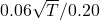$0.06\sqrt{T}/0.20$ :

Window	t-statistic	$P(\hat{\mu} > 0)$
10 years	0.95	82.9%
25 years	1.50	93.3%
36 years	1.80	96.4%
50 years	2.12	98.3%
100 years	3.00	99.9%

Fifty years of data to reach a t-statistic of two on the single most studied number in finance. And that is assuming the premium was constant throughout, which nobody believes.

Mean-variance optimisation inherits the worst input. Markowitz takes a covariance matrix and a vector of expected returns. One of those can be estimated well from a few years of daily data. The other cannot be estimated at all. Optimisers are notoriously sensitive to the expected-return vector, which is exactly the input carrying a three-percentage-point standard error after a career of observation. The instability is not a numerical artefact of the optimiser. It is the optimiser faithfully propagating the uncertainty it was handed.

And this is why option prices do not contain $\mu$

Here is the part that makes the whole thing cohere.

The Black-Scholes formula takes spot, strike, rate, time and volatility. The expected return of the underlying does not appear. Students find this bizarre and are usually told it follows from risk-neutral valuation, which is true and unsatisfying.

The statistical fact above is the other half of the answer. If $\mu$ did appear in the formula, every option price would depend on a parameter that nobody can measure — a quantity with a three-point standard error after 36 years of data. There would be no agreement on the price of a listed call, ever, because there is no agreement on $\mu$ and there cannot be.

Instead the price depends on $\sigma$ , which is pathwise observable and which the market quotes directly. A pricing theory whose inputs are all estimable is a theory that can produce a tradeable number. That is not a coincidence of the mathematics; it is the reason delta hedging is the right foundation.

The replication argument eliminates $\mu$ because $\mu$ is the one thing that could never have been pinned down.

What to do instead

Nobody gets to stop estimating expected returns — portfolios still have to be built. But the right posture changes.

Shrink hard towards a prior. If the data carries a three-point standard error, a sample mean deserves very little weight relative to a structural view. Black-Litterman is the standard machinery for this and its whole purpose is to stop the sample mean dominating.

Prefer methods that do not need the drift. Minimum-variance portfolios, risk parity and equal weighting all avoid the unestimable input and use only the one you can measure. Their empirical robustness is not mysterious: they are built from the parameter that the data actually identifies.

And treat any backtest that ranks strategies on realised mean return with the suspicion the 33.5% figure deserves.

The honest caveats

The $\sigma/\sqrt{T}$ result assumes a constant drift and constant volatility. Real volatility clusters and real expected returns almost certainly vary with the state of the economy. Both effects cut the same way: a time-varying drift is harder to pin down than a constant one, not easier, because the effective sample for any given regime is shorter than the calendar window.

There are genuine ways to do better, and they all work by bringing in information that is not in the price series. Cross-sectional structure, where thousands of assets share a few factors. Valuation ratios, which carry forward-looking information. Economic restrictions linking the premium to risk. None of them beats the bound above using the price path alone, because nothing can.

And the pathwise identification of $\sigma$ is a continuous-time idealisation. With real data, microstructure noise means the realised variance estimator stops converging and starts measuring the bid-ask bounce at high frequency. The asymmetry between the two parameters is real and enormous; the four decimal places are a model statement, not a trading-floor one.

The equivalence of measures that makes the drift unidentifiable is Girsanov’s theorem, and the second-order structure that makes volatility observable comes from Itô’s lemma.

Quadratic variation, change of measure and the reason pricing depends on one parameter and not the other are built up from first principles in the course modules.

Get the Quant Reference Card — four pages covering stochastic calculus, measure change, the models you’ll meet, discretisation, rates, credit and XVA. Free.