Every textbook on SDE discretisation gives you Euler-Maruyama first and then Milstein, with the note that Milstein is “first order” while Euler is “half order”, and moves on. What almost none of them tell you is when that upgrade is worth writing, when it does nothing at all, and when it fails to fix the problem you actually have.
The short version: the Milstein correction depends on the derivative of the volatility function. If your volatility doesn’t depend on the state, the extra term is identically zero and Milstein is Euler with more code. For sufficiently regular coefficients, the correction can improve strong convergence; the GBM experiment below illustrates this. For CIR near zero, the usual smoothness assumptions fail and the standard explicit correction is not a general positivity guarantee.
The two schemes
For a scalar SDE

Euler-Maruyama is the obvious discretisation, replacing differentials with increments:

Milstein adds one term:

These are scalar formulas. Standard strong-order results require suitable smoothness, growth and Lipschitz conditions on the coefficients, plus moment bounds. A nonzero sigma-prime alone does not establish order 1. In multiple dimensions, Milstein generally involves cross terms and iterated stochastic integrals; commutative noise can simplify them. CIR falls outside the usual globally Lipschitz diffusion assumptions.
Look at what that term contains. It is the product of the volatility and its own derivative with respect to the state, multiplied by  , which has mean zero and represents the difference between realised and expected quadratic variation over the step.
The correction exists because Euler treats  as frozen across the interval. It isn’t — as
 moves during the step, so does its volatility. Milstein picks up the first-order effect of that drift in volatility via a stochastic Taylor expansion. That is the entire idea.
Case 1: when it works
Geometric Brownian motion,  , so
 . Non-zero, so the correction is live.
Because GBM has an exact solution, we can drive both schemes with the same Brownian path and compare each against the truth. That measures strong error — pathwise accuracy,  — which is the thing these convergence orders refer to.
This independently specified benchmark uses S0=100, mu=0.05, sigma=0.20, T=1, 100,000 paths and seed 20261019. Each batch contains 2,000 paths; the same finest Brownian increments are aggregated across all grid levels. The complete code below reproduces this table and reports Monte Carlo standard errors.
| Steps | Euler terminal L1 error | Milstein terminal L1 error | Error ratio |
|---|---|---|---|
| 4 | 1.13681566 | 0.20689056 | 5.49 |
| 8 | 0.82056786 | 0.10703692 | 7.67 |
| 16 | 0.58462972 | 0.05457211 | 10.71 |
| 32 | 0.41714716 | 0.02756289 | 15.13 |
| 64 | 0.29624551 | 0.01387919 | 21.34 |
| 128 | 0.20977204 | 0.00696242 | 30.13 |
| 256 | 0.14823098 | 0.00348788 | 42.50 |
The local observed orders between 128 and 256 steps are approximately 0.501 for Euler and 0.997 for Milstein. At 256 steps the strong-error ratio is 42.50; this is not a speedup or a ratio of option-pricing errors.
An observed slope near 0.5 in an expected first-order experiment calls for investigation of regularity, coupling, the asymptotic grid range and Monte Carlo uncertainty, as well as the implementation. Matching one terminal mean does not establish weak convergence for general payoffs. The usual weak-order-one result requires additional coefficient and test-function assumptions; discontinuous or path-dependent payoffs need separate analysis.
Case 2: when it does nothing
For additive noise write  . Vasicek has
 , and Hull–White has
 . The state derivative of sigma is zero, so the scalar Milstein correction vanishes. Euler is exact at grid times for arithmetic Brownian motion with constant drift and volatility; it is not generally exact for Vasicek or Hull–White. Exact Gaussian transitions are available for these linear models.

Here  . The Milstein term is
 identically. Not small — zero.
The two displayed updates are algebraically identical for additive noise. No simulation is needed to establish that identity. With suitable smoothness and moment conditions, Euler can itself attain strong order one in the additive-noise setting.
This is worth internalising because a large fraction of rates modelling lives here. Vasicek, Hull-White, Ho-Lee, arithmetic Brownian motion — all constant-volatility, all immune to the upgrade. If someone tells you their Hull-White engine uses Milstein for accuracy, they have written a zero and multiplied by it.
The rule is simple: look at  before writing any code. If it’s zero, stop.
Case 3: when it doesn’t save you
CIR is where people reach for Milstein most, and where the story gets uncomfortable.

Here  , so
 — non-zero, so the correction is live, and it simplifies neatly since
 . The Milstein term becomes
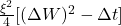 , with no square root in it at all.
The reason people want it: Euler on CIR generates negative rates, which is nonsense for a process that is provably non-negative. The hope is that Milstein fixes it.
The regularised derivative used here is not the derivative of the truncated diffusion, and its product does not equal  near zero. The simplified interior CIR Milstein term is
 , but applying it outside r>0 is a separate numerical extension and is not a positivity guarantee. Use a specifically defined and validated CIR scheme. Full truncation may keep an internal negative state; exact transition sampling is nonnegative at observation times.
The earlier CIR comparison table is withdrawn because its complete generating script and definition of the negative-state statistic were not specified. A terminal-state fraction and a fraction of time steps are different quantities. No claim about which scheme produces more negative values is made here without a reproducible experiment.
Matching a terminal mean alone does not demonstrate weak convergence. For boundary-sensitive payoffs, compare a fully specified scheme with exact grid transitions where available, and assess integration and monitoring errors separately.
Code
import numpy as np

def step(X, b, sigma, dsigma, dt, dW, milstein=False):
    """One step of Euler-Maruyama, or Milstein if the flag is set."""
    s = sigma(X)
    out = X + b(X)*dt + s*dW
    if milstein:
        out += 0.5*s*dsigma(X)*(dW**2 - dt)
    return out

# GBM: sigma(S) = 0.2*S, so dsigma(S) = 0.2  -> correction is live
gbm_sigma  = lambda S: 0.20*S
gbm_dsigma = lambda S: 0.20*np.ones_like(S)

# Vasicek: sigma(r) = 0.01 constant, so dsigma(r) = 0  -> correction is zero
vas_sigma  = lambda r: 0.01*np.ones_like(r)
vas_dsigma = lambda r: np.zeros_like(r)

# CIR requires a separately specified boundary-aware scheme.
Reproducible GBM benchmark
"""Independent specified benchmark, not reproduction of undocumented article tables.
Common Brownian paths for Euler, Milstein and exact GBM at each grid.
Same finest Brownian sample aggregated to all coarser grids, in memory-safe batches.
"""
import numpy as np
S0,mu,sigma,T=100.,.05,.2,1.
M,finest,batch=100_000,256,2000
levels=np.array([4,8,16,32,64,128,256])
rng=np.random.default_rng(20261019)
totals=np.zeros((len(levels),2)); squares=np.zeros_like(totals)
for start in range(0,M,batch):
    count=min(batch,M-start)
    increments=np.sqrt(T/finest)*rng.standard_normal((count,finest))
    exact=S0*np.exp((mu-.5*sigma**2)*T+sigma*increments.sum(axis=1))
    for i,n in enumerate(levels):
        dw=increments.reshape(count,n,finest//n).sum(axis=2);dt=T/n
        em=S0*np.prod(1+mu*dt+sigma*dw,axis=1)
        mil=S0*np.prod(1+mu*dt+sigma*dw+.5*sigma**2*(dw**2-dt),axis=1)
        errs=np.column_stack([abs(em-exact),abs(mil-exact)])
        totals[i]+=errs.sum(axis=0);squares[i]+=(errs**2).sum(axis=0)
means=totals/M
se=np.sqrt((squares-M*means**2)/(M-1)/M)
for n,errors,stderr in zip(levels,means,se):
    print(n,'L1 errors',errors,'SE',stderr,'ratio',errors[0]/errors[1])
print('Local observed orders',np.log2(means[:-1]/means[1:]))
print('These are terminal strong errors, not payoff errors, path-monitoring errors or speedups.')
Before writing any of this, evaluate symbolically. That single check tells you whether the rest is worth doing.
The decision, in practice
Is zero? Then Euler and Milstein are the same scheme. Vasicek, Hull-White, arithmetic Brownian motion. Write Euler and move on.
Do you need pathwise accuracy? Under the stated regularity conditions, scalar Milstein can improve strong order from 0.5 to 1. Validate that result for the model and quantity being estimated.
Do you only need expectations? Choose the scheme using measured computational cost for a target error in the quantity of interest. A ratio of pathwise errors is not a ratio of option-pricing errors or run times. Barrier and lookback payoffs also have monitoring bias. For a European claim under GBM, exact terminal simulation removes the SDE discretisation error altogether.
Is your problem a boundary? Use a specifically defined and validated boundary-aware scheme; standard explicit Milstein is not a general positivity guarantee.
The general point: Milstein is not a free upgrade, and it is not a fix for whatever is wrong with your simulation. It is a specific correction for a specific error term, and knowing which error you actually have is the whole of the decision.
Discretisation, strong versus weak convergence, and the numerical checks that tell you when a scheme is trustworthy are worked through from the ground up in the course modules.
Get the Quant Reference Card — four pages covering stochastic calculus, measure change, the models you’ll meet, discretisation, rates, credit and XVA. Free.