Variance Reduction in Monte Carlo: Which Technique When?

Monte Carlo error falls like $1/\sqrt{N}$ . To halve it you quadruple the paths, and past a certain point that stops being a strategy. Variance reduction techniques buy the same accuracy for fewer paths — sometimes by a factor of two, sometimes by a factor of five hundred.

But they are not interchangeable, and one of them makes things actively worse on payoffs where people apply it by habit. Here is which to reach for, with the measured factors.

The four you actually use

A one-million-path at-the-money call, $S_0 = K = 100$ , $r = 5\%$ , $\sigma = 20\%$ , $T = 1$ . Black-Scholes gives 10.4506.

Method	Estimate	Std error	Variance reduction
Plain Monte Carlo	10.4618	0.01473	1.0×
Antithetic variates	10.4454	0.01041	2.0×
Control variate (using $S_T$ )	10.4484	0.00561	6.9×

A 6.9× variance reduction means you need seven times fewer paths for the same accuracy. That is a real saving and it costs four lines of code.

Antithetic variates, and when they backfire

The idea: for every draw $Z$ , also use $-Z$ . Since the two are negatively related for a monotone payoff, their errors partly cancel.

The estimator is $\frac{1}{2}\left(f(Z) + f(-Z)\right)$ , whose variance is

$\frac{\operatorname{Var}(f) + \operatorname{Cov}\big(f(Z), f(-Z)\big)}{2}$

Two independent draws would give $\operatorname{Var}(f)/2$ . So antithetic sampling wins **if and only if that covariance is negative** — and that requires the payoff to be monotone in the driver.

Testing four payoffs on the same two million paths:

Payoff	corr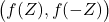 $\big(f(Z), f(-Z)\big)$	Variance ratio
Call, K=100	−0.5018	2.01×	helps
Put, K=100	−0.4151	1.71×	helps
Straddle at the forward	+0.8993	0.53×	hurts
Butterfly 90/100/110	+0.4289	0.70×	hurts

A straddle centred on the forward is nearly **symmetric** in $Z$ : an up-move and a down-move of the same size produce almost the same payoff. So $f(Z)$ and $f(-Z)$ are strongly *positively* correlated, the covariance term adds instead of cancelling, and you end up with roughly half the effective sample size you would have had by drawing independently.

Nobody notices, because the estimate is still unbiased and converges. It just converges more slowly than doing nothing clever, which is the worst kind of bug: it looks like it is working.

**The test before you apply it:** is the payoff monotone in the underlying random driver? Calls, puts, digitals, barriers in one direction — yes. Straddles, butterflies, strangles, anything V-shaped or symmetric — no. If in doubt, measure the correlation between $f(Z)$ and $f(-Z)$ on a small sample. It takes one line and it is definitive.

Control variates, the reliable workhorse

If you know a quantity $X$ whose expectation you can compute exactly, and it correlates with your payoff, use it to correct the estimate:

$\hat{V} = \frac{1}{N}\sum \left[ f(Z_i) - b\left(X_i - \mathbb{E}[X]\right) \right]$

The correction has expectation zero, so the estimator stays unbiased. The optimal coefficient is

$b^* = \frac{\operatorname{Cov}(f, X)}{\operatorname{Var}(X)}$

and the variance falls by a factor $1/(1-\rho^2)$ where $\rho$ is the correlation between payoff and control.

For a call, the natural control is the discounted stock itself, because $\mathbb{E}[e^{-rT}S_T] = S_0$ exactly by construction. That is free information you already have and are otherwise throwing away. On the run above the optimal $b$ came out at 0.6739 and bought a **6.9× variance reduction** — better than antithetic, and it works regardless of payoff shape.

The general recipe: find a related instrument you can price in closed form. A geometric-average Asian for an arithmetic one. A Black-Scholes vanilla for a stochastic-volatility vanilla. A European for a Bermudan. The closer the correlation, the bigger the win, and unlike antithetic sampling it degrades gracefully — a weak control just does less, it does not hurt.

Importance sampling, when the payoff is rare

This is the one with the dramatic numbers, and it matters for exactly the cases where plain Monte Carlo falls apart.

Price a deeply out-of-the-money call, $K = 180$ , true value 0.028643:

Method	Estimate	Std error	Paths finishing ITM	Variance reduction
Plain Monte Carlo	0.029093	0.000809	0.269%	1×
Importance sampling	0.028676	0.000036	50.1%	510×

Plain Monte Carlo throws away 99.7% of its work. A million paths and only 2,700 contribute anything; the rest return zero and just add noise.

Importance sampling shifts the sampling distribution so the strike sits in the middle of it — here, a drift shift that puts half the paths in the money — and then corrects the bias by weighting each path:

$w = \exp\left(-\mu_s Z - \frac{1}{2}\mu_s^2\right)$

That weight is a Radon-Nikodym derivative. Importance sampling and risk-neutral pricing are the same operation pointed at different goals: one reweights to remove a risk premium, the other reweights to sample the region you care about. Recognising that makes both easier to implement and easier to debug.

A 510× variance reduction is equivalent to running 510 million paths instead of one million. There is no amount of extra compute that competes with picking the right sampling distribution.

**Where it matters in practice:** tail risk, deep out-of-the-money options, default probabilities, credit losses, PFE at high quantiles. Anywhere the interesting event is rare, plain Monte Carlo is mostly sampling nothing.

**The one caution:** if you shift too aggressively, the weights become extremely dispersed and the estimator degrades — the same failure mode as an over-stretched change of measure. The rule of thumb that works is to centre the sampling distribution on the region of interest, not beyond it.

Quasi-Monte Carlo, briefly

Worth knowing it exists. Replace pseudo-random numbers with low-discrepancy sequences — Sobol, Halton — which fill the space more evenly. The convergence rate improves from $O(N^{-1/2})$ towards roughly $O(N^{-1})$ for problems with low effective dimension.

The catch is that dimension. Sobol works beautifully for a European option with one time step and poorly for a path-dependent payoff with 252 of them, unless you reorder the dimensions so the most important ones come first — the Brownian bridge or PCA construction. That reordering is where the skill lives, and it is why QMC is often skipped: the technique is easy, the setup is not.

Which to use, in order

**Start with a control variate.** It is the most robust, it never makes things worse, and there is almost always a related instrument with a closed form. It is the first thing to reach for and often enough on its own.

**Add antithetic variates only if the payoff is monotone.** Free 2×, one line of code. But check the monotonicity first, because on a symmetric payoff you are halving your effective sample size while believing you have doubled it.

**Use importance sampling when the event is rare.** This is where the order-of-magnitude wins are. If fewer than a few percent of your paths contribute, nothing else will help comparably.

**Consider QMC when the effective dimension is low**, and expect to spend the time on the dimension ordering rather than on the sequence itself.

And they combine. Control variates plus antithetic on a monotone payoff is routine and multiplicative.

Code

import numpy as np

S0, K, r, sig, T, M = 100., 100., 0.05, 0.20, 1.0, 1_000_000
rng = np.random.default_rng(2)
Z = rng.standard_normal(M)
disc = np.exp(-r*T)
ST = lambda z: S0*np.exp((r - 0.5*sig**2)*T + sig*np.sqrt(T)*z)

payoff = disc*np.maximum(ST(Z) - K, 0)

# --- control variate: E[disc * S_T] = S0, known exactly ---
X = disc*ST(Z)
b = np.cov(payoff, X)[0, 1]/np.var(X)
cv = payoff - b*(X - S0)
print(f"plain    {payoff.mean():.4f}  se {payoff.std(ddof=1)/np.sqrt(M):.5f}")
print(f"control  {cv.mean():.4f}  se {cv.std(ddof=1)/np.sqrt(M):.5f}")

# --- the antithetic check you should always run first ---
h = M//2
a, bb = disc*np.maximum(ST(Z[:h]) - K, 0), disc*np.maximum(ST(-Z[:h]) - K, 0)
print(f"corr(f(Z), f(-Z)) = {np.corrcoef(a, bb)[0,1]:+.4f}"
      f"   -> {'use antithetic' if np.corrcoef(a,bb)[0,1] < 0 else 'DO NOT'}")

That last check is three lines and it is the one people skip. Negative correlation means antithetic sampling helps; positive means it is costing you paths.

The takeaway

Variance reduction is not one technique with a dial. Control variates are the safe default and buy about 7× on a vanilla call. Antithetic variates buy 2× on monotone payoffs and cost you nearly half your sample on symmetric ones. Importance sampling buys 500× on rare events and nothing at all on ordinary ones.

The skill is matching the technique to the shape of the problem — and the shape is usually obvious once you ask whether the payoff is monotone, whether you know a related closed form, and whether most of your paths are contributing anything at all.

Worth reading alongside Monte Carlo option pricing in Python for the base implementation, Euler vs Milstein for the discretisation error that variance reduction does not fix, and the Radon-Nikodym derivative, which is the same object doing the work inside importance sampling.

Monte Carlo construction, discretisation and the numerical checks that tell you when an estimator is trustworthy are worked through from the ground up in the course modules.

Get the Quant Reference Card — four pages covering stochastic calculus, measure change, the models you'll meet, discretisation, rates, credit and XVA. Free.